library(tidyverse)Solution
How to do it correctly
After reading the instruction of the exercise session, this page is going to show you how the exercise should work step by step. Note that it’s possible to find an error and your code is not working the way it should be. First, make sure you have followed the steps correctly. Re-examine the code, perhaps you missed something even one word or punctuation. Read the error, it helps you to find the exact mistake you made in the code.
First Prep
Remember the first step in the lecture session? Always load the package to make the functions work. We need to load some packages before started to make any models.
tidyverse is going to help you read the data in certain format, such as .csv.
Call the Data
We need to call the data we’re going to use with the function in the tidyverse package.
pisa <- read.csv("../dataset/pisa_idn_sample.csv")read.csv function calls the data in .csv format. The other things before the slash is the name of the data being placed. While the ../ is a html command to call the data in different folder. In this case, dataset folder is not in the same folder with this page.
Random Intercept Model
Begin Modeling
Before we’re stepping into modeling, make sure we load the package to run the multilevel model function.
library(lme4)Next step is modeling random intercept:
m1 <- lmer(MATH ~ 1 + growth + (1 | CNTSCHID), data = pisa)If you have created the model, now you can see the result by calling it with summary.
View the Result
summary(m1)Linear mixed model fit by REML ['lmerMod']
Formula: MATH ~ 1 + growth + (1 | CNTSCHID)
Data: pisa
REML criterion at convergence: 13583.1
Scaled residuals:
Min 1Q Median 3Q Max
-2.7730 -0.6292 -0.0256 0.6266 4.4737
Random effects:
Groups Name Variance Std.Dev.
CNTSCHID (Intercept) 2083 45.64
Residual 1874 43.29
Number of obs: 1297, groups: CNTSCHID, 41
Fixed effects:
Estimate Std. Error t value
(Intercept) 354.774 7.373 48.121
growth 25.891 2.613 9.907
Correlation of Fixed Effects:
(Intr)
growth -0.122If you want to make the result into a table, then you need function tab_model. Make sure you load sjPlot package to run the function.
library(sjPlot)

tab_model(m1)| MATH | |||
|---|---|---|---|
| Predictors | Estimates | CI | p |
| (Intercept) | 354.77 | 340.31 – 369.24 | <0.001 |
| growth | 25.89 | 20.76 – 31.02 | <0.001 |
| Random Effects | |||
| σ2 | 1874.27 | ||
| τ00 CNTSCHID | 2082.74 | ||
| ICC | 0.53 | ||
| N CNTSCHID | 41 | ||
| Observations | 1297 | ||
| Marginal R2 / Conditional R2 | 0.037 / 0.544 | ||
Visualise Model in ggplot
This step guide you to visualise the model you have created into a plot.
pisa$m1 <- predict(m1)

pisa |>
  ggplot(aes(growth, m1, color = CNTSCHID, group = CNTSCHID)) +
  geom_smooth(se = F, method = lm) +
  theme_bw() +
  labs(x = "Growth Mindset",
       y = "Mathematic",
       color = "CNTSCHID")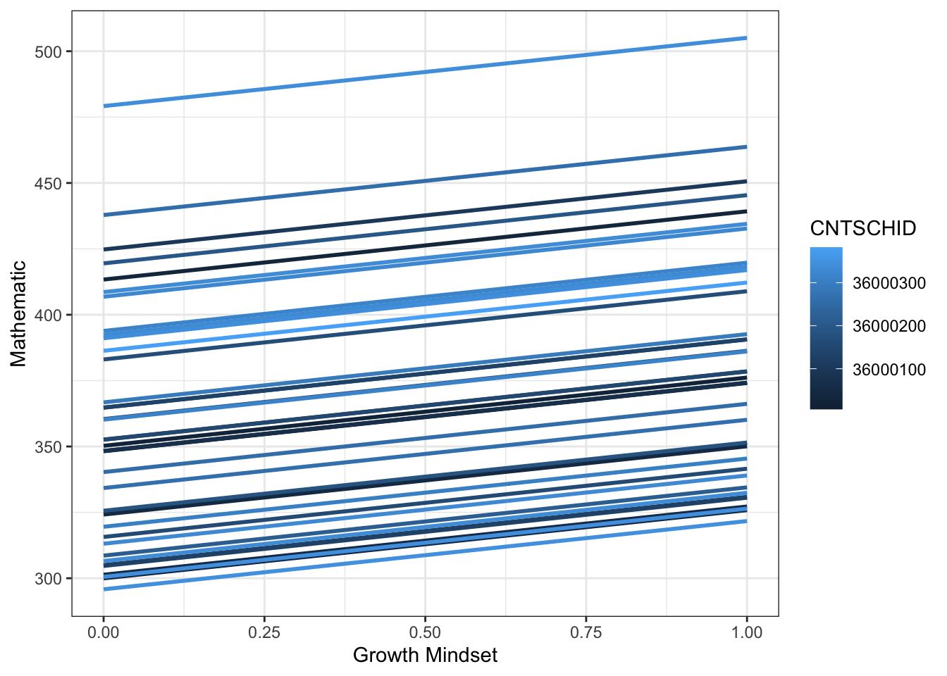
Visualise Model in qqmath
library(lattice)

qqmath(ranef(m1, condVar = TRUE))
$CNTSCHID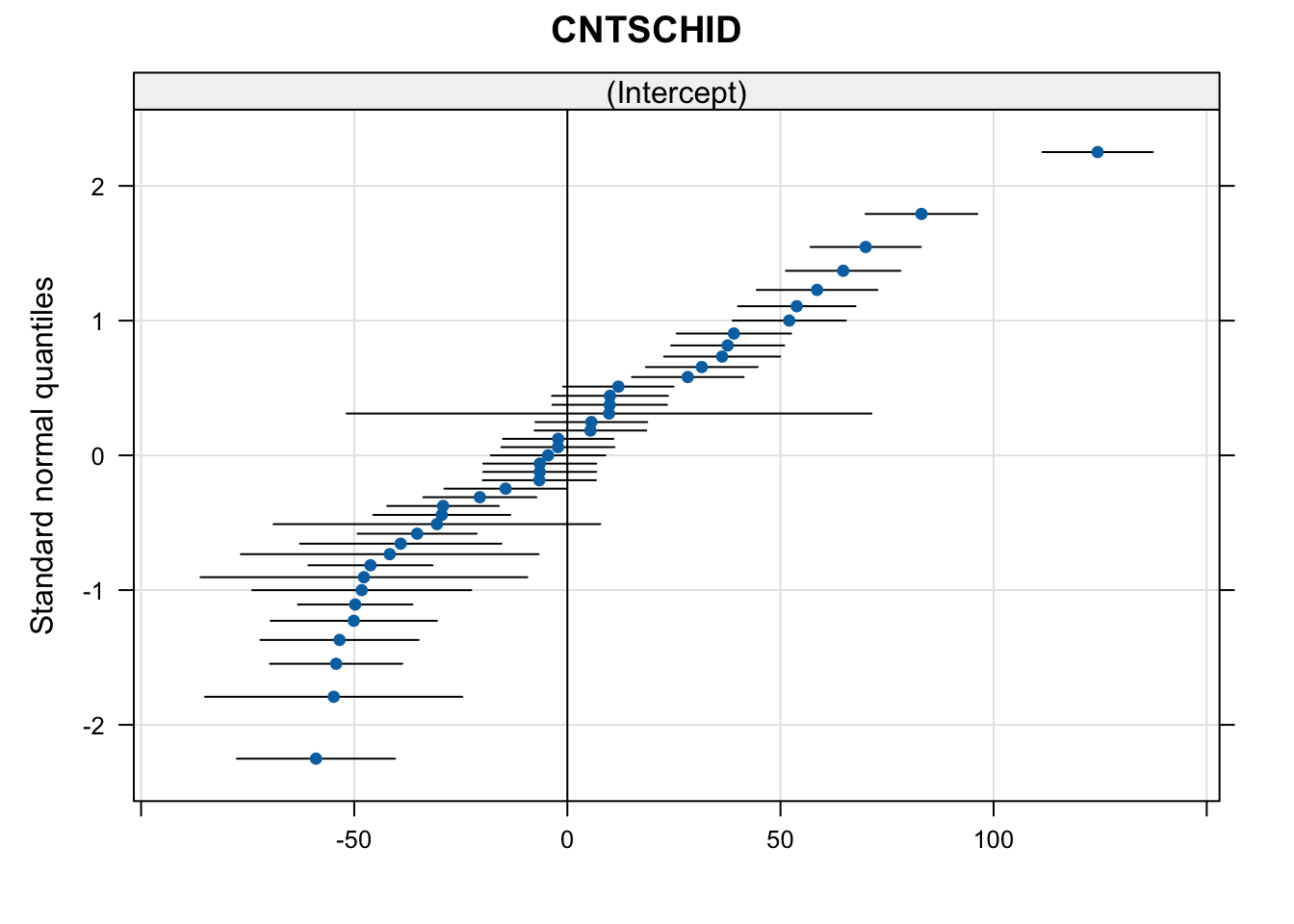
Random Slope Model
Following the steps above is going to make random slope model easier. Although it is not the same model, the steps quite familiar and same packages used. We don’t need to load the packages that we have loaded before. Now, it’s just modeling, viewing, and visualise the model.
Modeling
m2 <- m2 <- lmer(MATH ~ 1 + ESCS + (1 + ESCS | CNTSCHID), data = pisa)Viewing
We’re going to see the result with summary and tab_model to see the model in table form.
Summary
summary(m2)Linear mixed model fit by REML ['lmerMod']
Formula: MATH ~ 1 + ESCS + (1 + ESCS | CNTSCHID)
Data: pisa
REML criterion at convergence: 13653.8
Scaled residuals:
Min 1Q Median 3Q Max
-2.8809 -0.6318 -0.0380 0.6109 4.1509
Random effects:
Groups Name Variance Std.Dev. Corr
CNTSCHID (Intercept) 2996.20 54.738
ESCS 61.09 7.816 0.79
Residual 1961.08 44.284
Number of obs: 1297, groups: CNTSCHID, 41
Fixed effects:
Estimate Std. Error t value
(Intercept) 367.305 9.069 40.503
ESCS 3.352 1.948 1.721
Correlation of Fixed Effects:
(Intr)
ESCS 0.682 Table
tab_model(m2)| MATH | |||
|---|---|---|---|
| Predictors | Estimates | CI | p |
| (Intercept) | 367.30 | 349.51 – 385.10 | <0.001 |
| ESCS | 3.35 | -0.47 – 7.17 | 0.086 |
| Random Effects | |||
| σ2 | 1961.08 | ||
| τ00 CNTSCHID | 2996.20 | ||
| τ11 CNTSCHID.ESCS | 61.09 | ||
| ρ01 CNTSCHID | 0.79 | ||
| ICC | 0.53 | ||
| N CNTSCHID | 41 | ||
| Observations | 1297 | ||
| Marginal R2 / Conditional R2 | 0.003 / 0.528 | ||
Visualise
Here, we’re going to visualise the model through ggplot and qqmath.
pisa$m2 <- predict(m2)

pisa %>%
  ggplot(aes(ESCS, m1, color = CNTSCHID, group = CNTSCHID)) +
  geom_smooth(se = F, method = lm) +
  theme_bw() +
  labs(x = "ESCS",
       y = "Matematika",
       color = "CNTSCHID")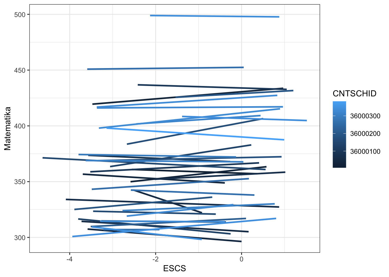
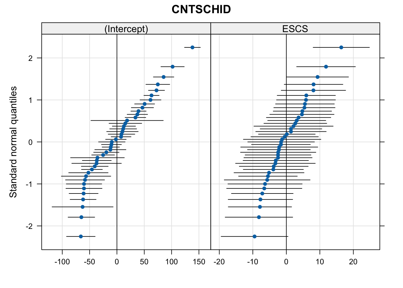
qqmath(ranef(m2, condVar = TRUE))$CNTSCHID