     vars    n   mean    sd median trimmed   mad    min    max  range skew
ESCS    1 1297  -1.49  1.04  -1.56   -1.51  1.00  -4.63   1.52   6.15 0.18
MATH    2 1297 374.02 64.42 365.02  370.49 64.62 188.95 632.92 443.98 0.51
     kurtosis   se
ESCS    -0.34 0.03
MATH -0.04 1.79Simple Linear Regression
Introduction
- Statistical model is quite important across a wide range of fields, providing researchers with tools for both explanation and prediction.
- The most popular models of the statistical practice has been the general linear model (GLM).
- The GLM finds the relation of a dependent and several independents variables that take form of tools as analysis of variance (ANOVA) and regression.
Simple Linear Regression
- The simple linear regression model in population form is where \(y_i\) is the dependent variable for individual \(i\) in the data set and \(x_i\) is the independent variable for subject \(i\) (\(i\) = 1, …, \(N\)).
- The terms \(\beta_0\) dan \(\beta_1\), are the intercept and slope of the model, respectively.
\[ y=\beta_{0}+\beta_{1}X_i+\varepsilon_i{} \qquad(1)\]
- The intercept is the point at which the line in Equation 1 crosses the \(y\) axis at \(x\) = 0.
- Thus, larger values of \(\beta_1\) (positive or negative) indicate a stronger linear relationship between \(y\) and \(x\).
Ilustration of Simple Regression
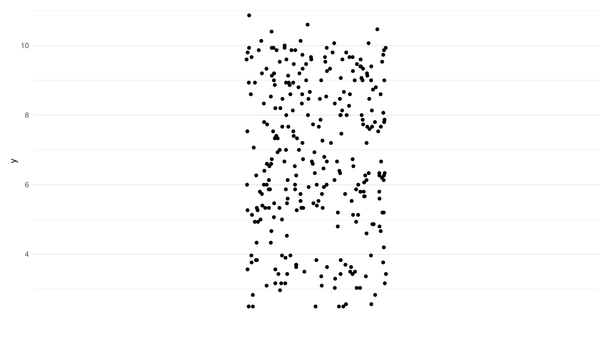
Imagine we have a dependent variable (y).
Ilustration of Simple Regression
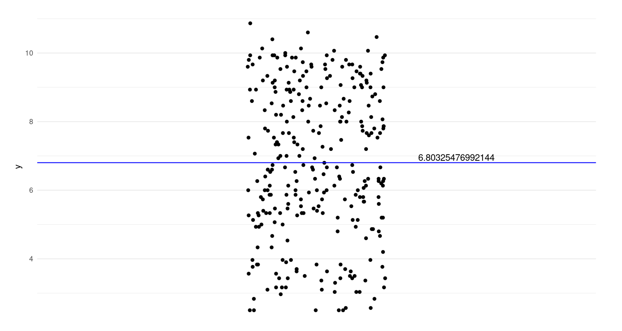
We estimate a linear regression with no predictors and plot the intercept (null model).
\[ y = \beta_0 + \varepsilon_i{} \]
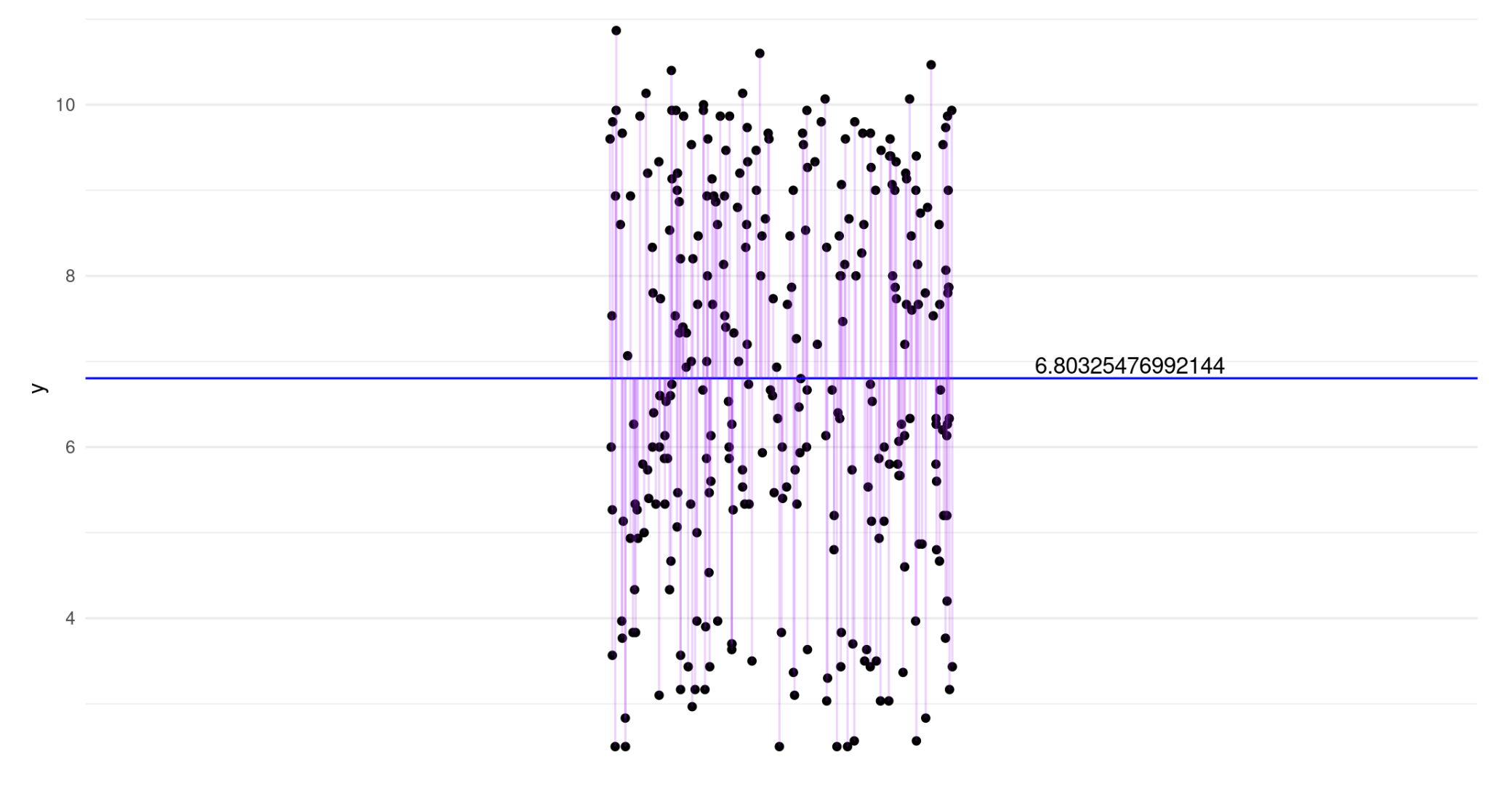
Ilustration of Random Error
- Purple lines indicate the error term for each observation.
Random Error
- Random error, represented by \(\varepsilon_i\), is inherent in any statistical model, including regression.
- It expresses the fact that for any individual, \(i\), the model will not generally provide a perfect predicted value of \(y\), denoted \(\hat{y}_i\) and obtained by applying the regression model as
\[ \hat{y} = \beta_0 + \beta_iX_i \qquad(2)\]
- Conceptually, this random error is representative of all factors that may influence the dependent variable other than \(x\).
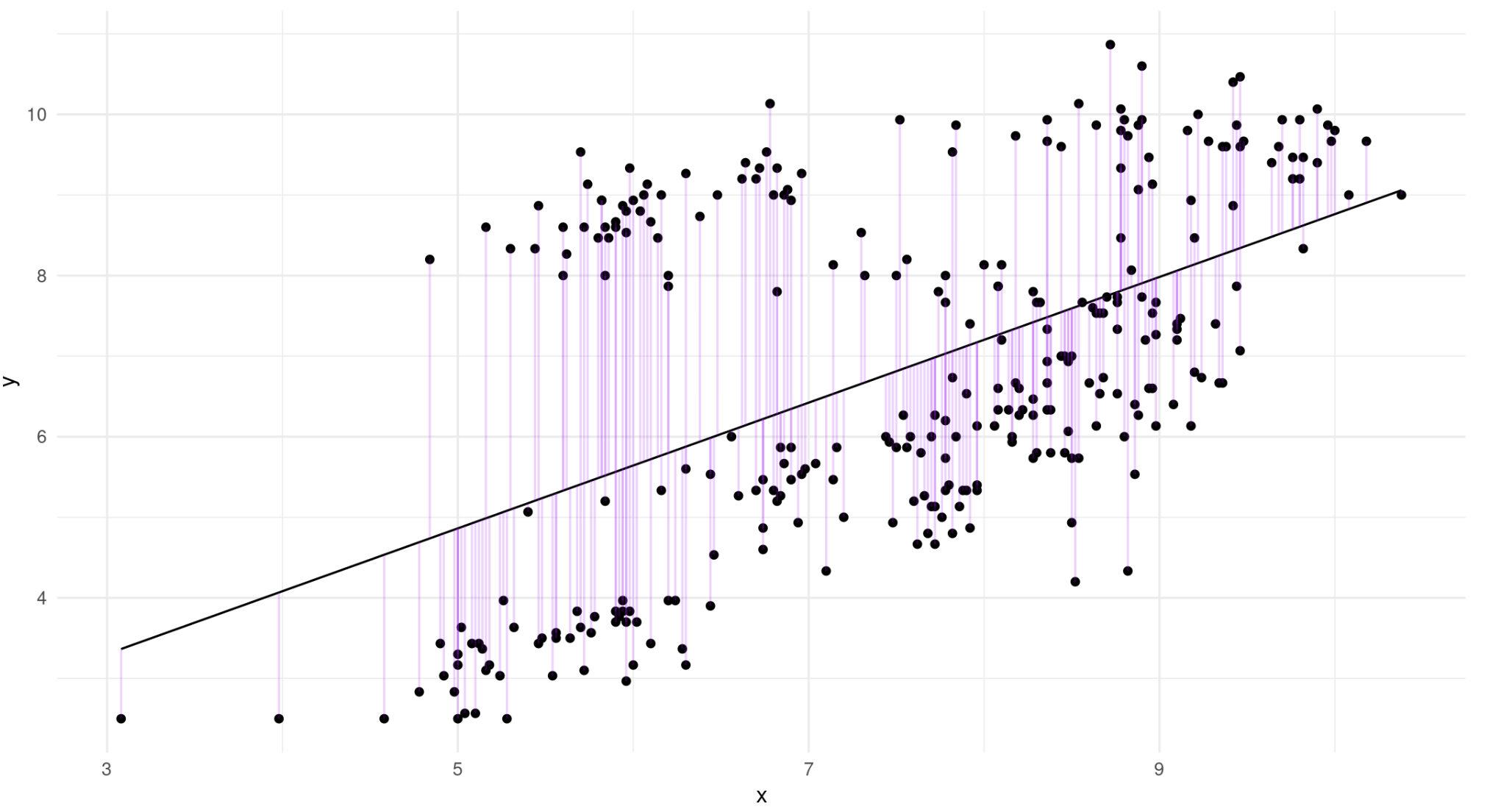
Ilustration of Simple Regression
\[ y = \beta_0 + \beta_iX_i + \varepsilon_i{} \]
Estimating Regression with OLS
- Ordinary least squares (OLS) is popular methods for obtaining estimated values of the regression model parameters (\(b_0\) and \(b_i\), respectively) given a set of \(x\) and \(y\).
- \(\beta_0\) and \(\beta_i\) must be estimated using sample data taken from the population.
- The goal of OLS is to minimize the sum of the squared differences between the observed values of \(y\) and the model-predicted values of \(y\), across the sample.
- This difference, known as the residual, is written as
\[ e_i = y_i - \hat{y}_i \qquad(3)\]
- Therefore, the method OLS seeks to minimize
\[ \Sigma_{i=1}^n e_i^2 = \Sigma_{i=1}^n (y_i - \hat{y}_i) \qquad(4)\]
OLS Criteria
- It should be noted that in the context of simple linear regression, the OLS criteria reduce to the following equations, which can be used to obtain \(b_0\) and \(b_i\) as
\[ \beta_0 = r \left(\frac{S_y}{S_x} \right) \qquad(5)\]
and
\[ \beta_0 = \overline{y} - \beta_1\overline{x} \qquad(6)\]
Example of Simple Regression
- In this example, we use the PISA 2022 data to analyze the impact of ESCS on the math achievement of Indonesian students.
- The sample includes 1329 students who were assessed for both variables.
- In this scenario, math achievement serves as the dependent variable, while ESCS is the independent variable.
- Descriptive statistics for each variable, along with the correlations between them, are provided in Table 1.1.
Descriptive stat
Correlation
| Variable | Mean | Standar Deviasi | Correlation |
|---|---|---|---|
| Math | 367.28 | 58.34 | 0.244 |
| ESCS | -1.63 | 0.99 |
Beta 1
- Using equations (1.4) and (1.5), we can use this information to obtain estimates for both the slope and the intercept of the regression model.
- First, the slope of the regression is calculated as
\[ \beta_1 = 0.244 \left(\frac{58.34}{0.99} \right)=14.38 \qquad(7)\]
Beta 0
The results indicate that individuals with higher ESCS scores generally achieve higher math scores.
We can calculate an estimate of the intercept using the values in the table:
\[ \beta_0 = \overline{y} - \beta_1\overline{x} \qquad(8)\]
\[ \beta_0 = 367.28-(14.38)(-1.63)=390.72 \]
Full model
- The resulting estimated regression equation for math and ESCS is:
\[ \hat {math}=390.72+14.38(ESCS). \]
- This indicates that for a 1-point increase in ESCS score, math achievement would increase by 390.72 points.
Measure the strength
- To assess the strength of the relationship between ESCS and math achievement, we should calculate the coefficient of determination.
- This requires the values of \(SS_R\) and \(SS_T\).
- The sum of squares due to regression (\(SS_R\)) or explained sum of squares (ESS) is the sum of the differences between the predicted value and the mean of the dependent variable.
Sum of squares due to regression
- We can calculate the strength by this equation.
\[SS_R=\Sigma^n_{i=1}(\hat{y}_i-\bar{y})^2\]
- Where \(\hat{y}_i\) is the predicted value of the dependent variable and \(\bar{y}\) is mean of the dependent variable.
Sum of squares error
- The sum of squares error (\(SS_E\)) or residual sum of squares is the difference between the observed and predicted values.
\[SS_E=\Sigma^n_{i=1}\varepsilon^2_i\] Where \(\varepsilon_i\) is the difference between the actual value of the dependent variable and the predicted value:
\[\varepsilon_i=y_i-\hat{y}_i\]
Sum of squares total
- The sum of squares total (\(SS_T\)) or the total sum of squares (TSS) is the sum \(SS_R\) and \(SS_E\).
\[SS_T=\Sigma^n_{i=1}(\hat{y}_i-\bar{y})^2 +\Sigma^n_{i=1}\varepsilon^2_i\]
Regression in R
To simplify the calculation we will calculate the \(R^2\) value using r. First, we create a regression model using the lm () function.
Calculate by hand
- We calculate the \(SS_R\), \(SS_E\), \(SS_T\), \(R^2\) value with the following command:
Calculate R square
\[ R^2=\frac{SS_R}{SS_T}= \frac{269424.3}{4520484}=0.06 \]
- The results indicate that about 6% of the difference in math achievement can be accounted for by the variance in ESCS scores.
Calculate F
- With this \(R^2\) value, we can compute the F-statistic to test if any of the model slopes (in this instance, there is only one) are different from 0 in the population.
\[ F= (\frac {1329-1-1} {1})(\frac{0.06}{1-0.06})= 84.7 \]