Hands-on Random Slope

Practice

Random Slope

  • The previous model makes the assumption that the effect of growth mindset is the same across all schools (that’s why the lines are parallel).

  • What if one growth mindset score is more ‘effective’ in some schools than others in improving maths scores.

  • At this point a random slope is needed.

  • We get a new coefficient that describes the differences between schools in the effect of growth mindset on maths scores.

Random Slope Estimation

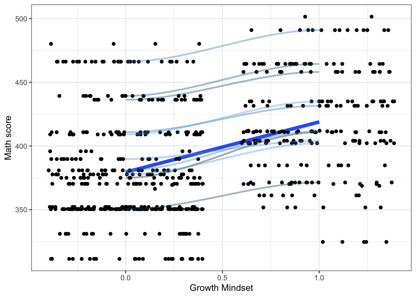
# model with random slope
m2 <- lmer(MATH ~ 1 + growth + 
             (1 + growth | CNTSCHID), 
           data = skor)
# print results
summary(m2)
Linear mixed model fit by REML ['lmerMod']
Formula: MATH ~ 1 + growth + (1 + growth | CNTSCHID)
   Data: skor

REML criterion at convergence: 6742.1

Scaled residuals: 
    Min      1Q  Median      3Q     Max 
-2.5923 -0.7214 -0.0927  0.6729  3.7811 
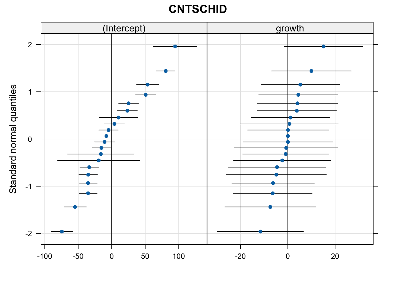
Random effects:
 Groups   Name        Variance Std.Dev. Corr
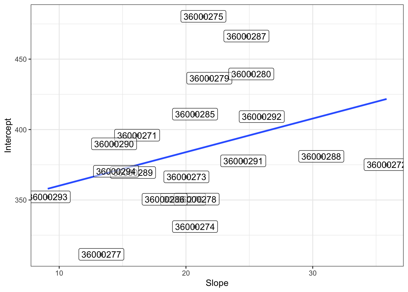
 CNTSCHID (Intercept) 2081.8   45.63        
          growth       126.2   11.23    0.14
 Residual             1876.3   43.32        
Number of obs: 644, groups:  CNTSCHID, 20

Fixed effects:
            Estimate Std. Error t value
(Intercept)  385.608     10.652  36.201
growth        20.687      4.692   4.409

Correlation of Fixed Effects:
       (Intr)
growth -0.026

Random Slope Estimation

tab_model(m2, show.icc = TRUE)
  MATH
Predictors Estimates CI p
(Intercept) 385.61 364.69 – 406.52 <0.001
growth 20.69 11.47 – 29.90 <0.001
Random Effects
σ2 1876.27
τ00 CNTSCHID 2081.84
τ11 CNTSCHID.growth 126.17
ρ01 CNTSCHID 0.14
ICC 0.54
N CNTSCHID 20
Observations 644
Marginal R2 / Conditional R2 0.024 / 0.548

Interpretation

  • The fixed effect of growth mindset is smaller than in model 1 and we have a new random effect coefficient.
  • The random slope variance for years of education is 73.29.

Density

skor$m2 <- predict(m2)
# visualize the predictions based on our model
skor %>% 
  ggplot(aes(growth, m2)) + 
  geom_smooth(se = F, method = lm, size = 2) +
  geom_jitter()+
  stat_smooth(aes(color = CNTSCHID, group = CNTSCHID),
              geom = "line", alpha = 0.4, size = 1) +
  theme_bw() +
  guides(color = F) +
  labs(x = "Growth Mindset", 
       y = "Math score", 
       color = "School")

Density Result

Fixed effect is -8.054, but each school has a diverse slope.

Density of Intercept

# another way to see random effect
qqmath(ranef(m2, condVar = TRUE))[[1]]

The graph shows how the influence of growth mindset varies across schools.

Random Effects

coefs_m2 <- coef(m2)

coefs_m2$CNTSCHID %>%
  mutate(CNTSCHID = rownames(coefs_m2$CNTSCHID))  %>% 
  ggplot(aes(growth, `(Intercept)`, label = CNTSCHID)) + 
  geom_point() + 
  geom_smooth(se = F, method = lm) +
  geom_label(nudge_y = 0.15, alpha = 0.5) +
  theme_bw() +
  labs(x = "Slope", y = "Intercept")

Interpretation

  • The graph shows that some schools have high maths scores but low effects on outcomes and vice versa.

  • The blue line represents the relationship between the random intercept and the slope with a coefficient of 0.6. This shows that the smaller the fixed mindset, the higher the maths score.