Hands-on Random Intercept

Practice

Creating Random Intercept Model

If we have previously created a null model without predictors, in the random intercept model we will include predictors. For example, if we want to know the relationship between ESCS and maths achievement, we can easily create the model with the same steps as when we created the null model.

m1 <- lmer(MATH ~ 1 + ESCS + (1 | CNTSCHID), data = pisa)

The result

summary(m1)

Linear mixed model fit by REML ['lmerMod']
Formula: MATH ~ 1 + ESCS + (1 | CNTSCHID)
   Data: pisa

REML criterion at convergence: 13670.3

Scaled residuals: 
    Min      1Q  Median      3Q     Max 
-3.0591 -0.6366 -0.0336  0.6187  4.5086 

Random effects:
 Groups   Name        Variance Std.Dev.
 CNTSCHID (Intercept) 2184     46.73   
 Residual             2004     44.77   
Number of obs: 1297, groups:  CNTSCHID, 41

Fixed effects:
            Estimate Std. Error t value
(Intercept)  370.330      7.833  47.280
ESCS           4.326      1.474   2.934

Correlation of Fixed Effects:
     (Intr)
ESCS 0.290

ICC result

tab_model(m1)

	MATH
Predictors	Estimates	CI	p
(Intercept)	370.33	354.96 – 385.70	<0.001
ESCS	4.33	1.43 – 7.22	0.003
Random Effects
σ²	2004.21
τ₀₀ _CNTSCHID	2183.92
ICC	0.52
N _CNTSCHID	41
Observations	1297
Marginal R² / Conditional R²	0.005 / 0.524

Prediction plot

pisa$m1 <- predict(m1)

pisa %>% 
  ggplot(aes(ESCS, m1, color = CNTSCHID, group = CNTSCHID)) + 
  geom_smooth(se = F, method = lm) +
  theme_bw() +
  labs(x = "ESCS", 
       y = "Matematika", 
       color = "CNTSCHID")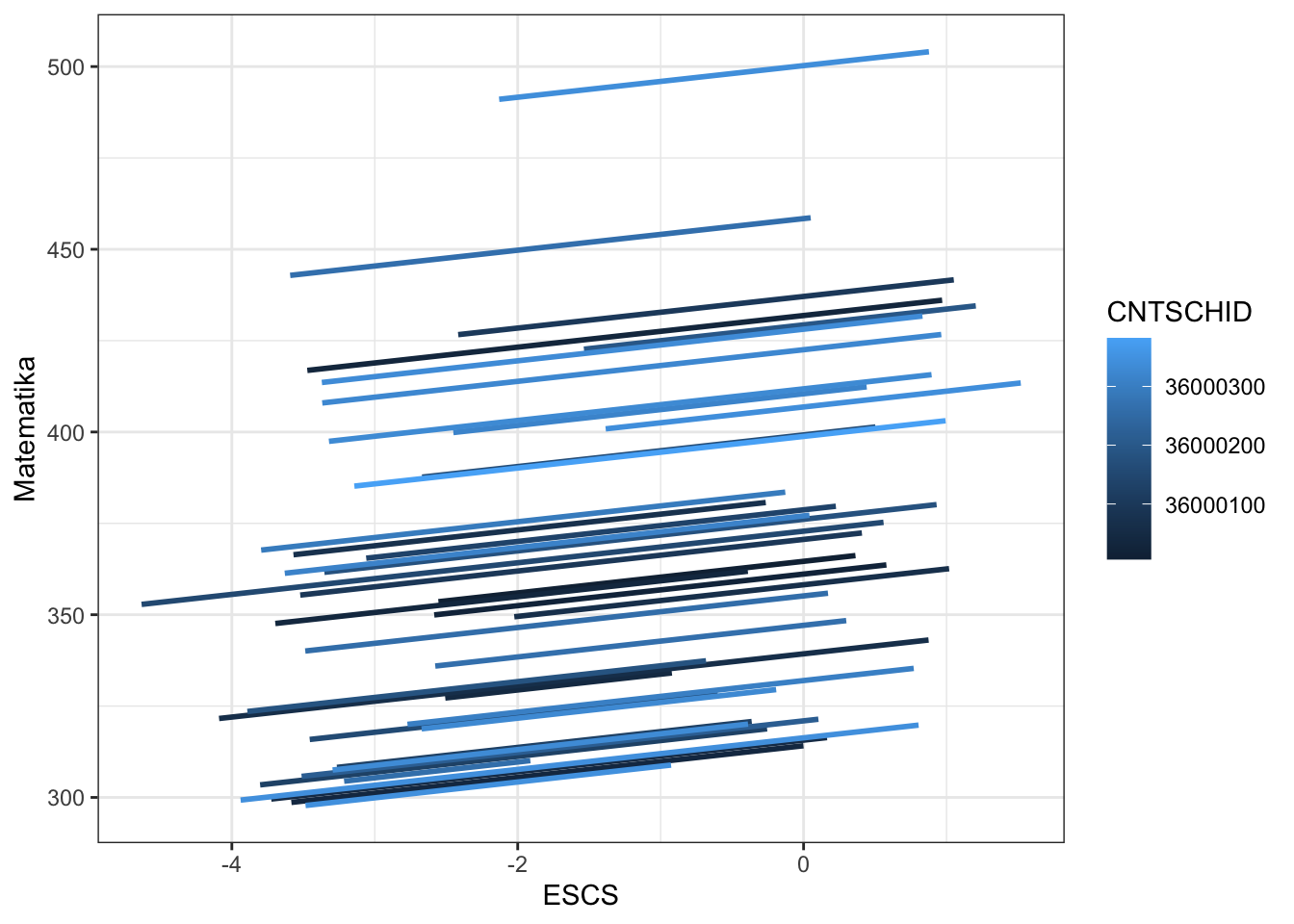

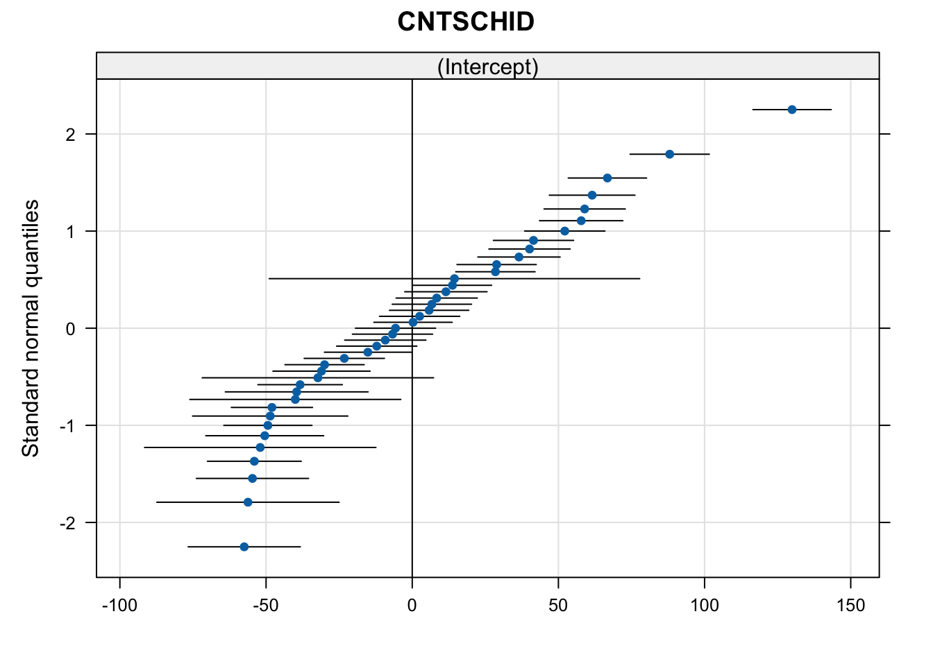
QQ-plot

qqmath(ranef(m1, condVar = TRUE))

$CNTSCHID