Random Slope
Intuition
Visual explanation
More real and visual explanation
Towards Random Slope
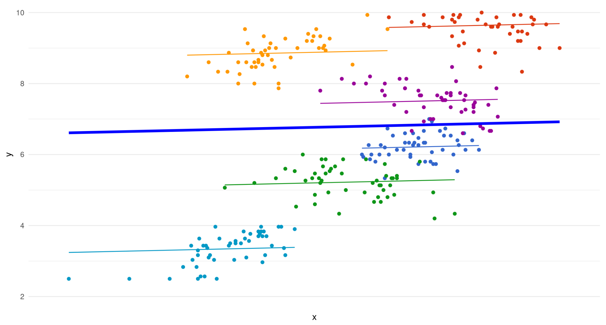
First, let’s consider the random-intercept, fixed slope model again.
All slopes are held constant, i.e. in each group we assume the same effect of x on y.
Is this really a reasonable assumption?
Towards Random Slope
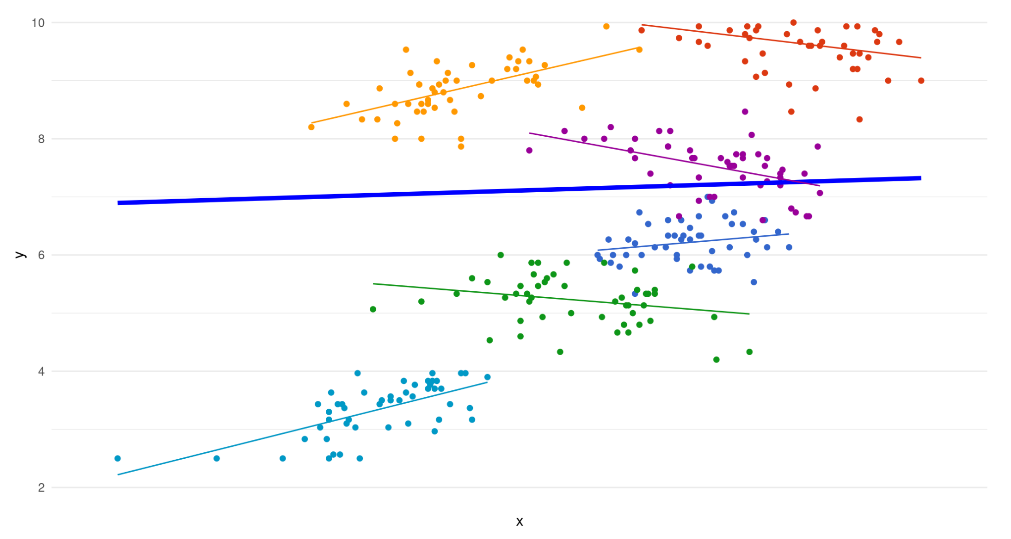
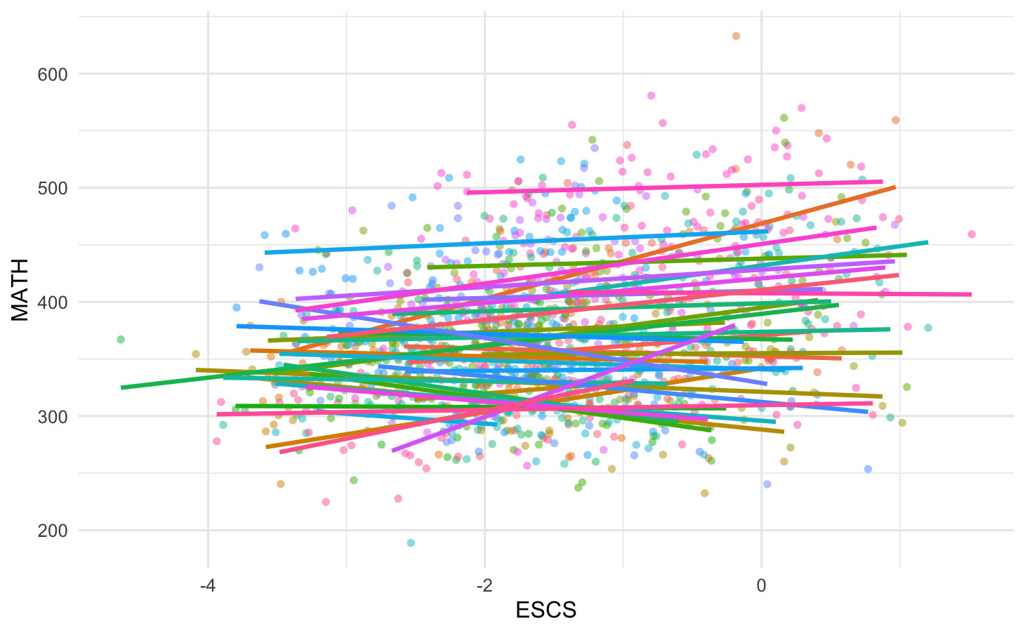
Instead we may introduce random slopes and let the slope vary by group.
We can see that it some groups the relationship is differs in strength or even becomes negative when allowing the slopes to vary.
Towards Random Slope
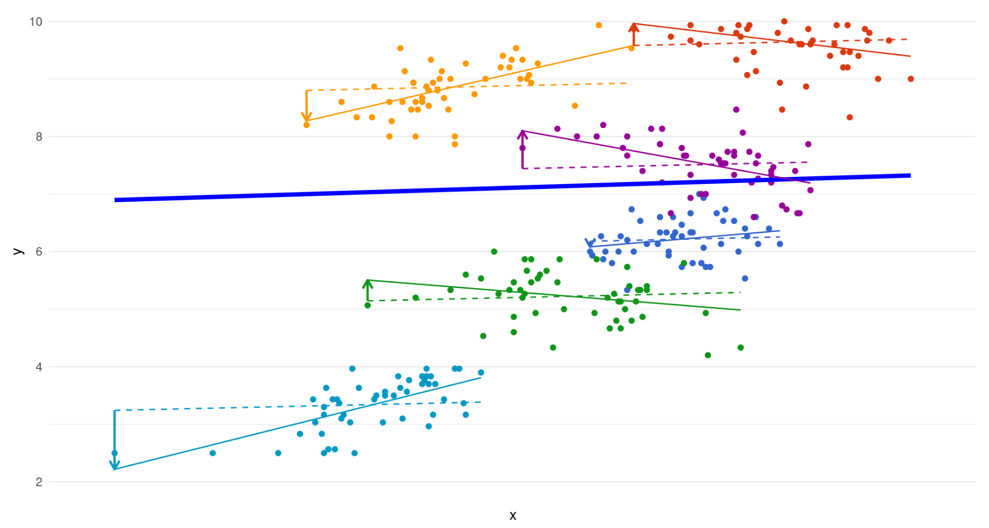
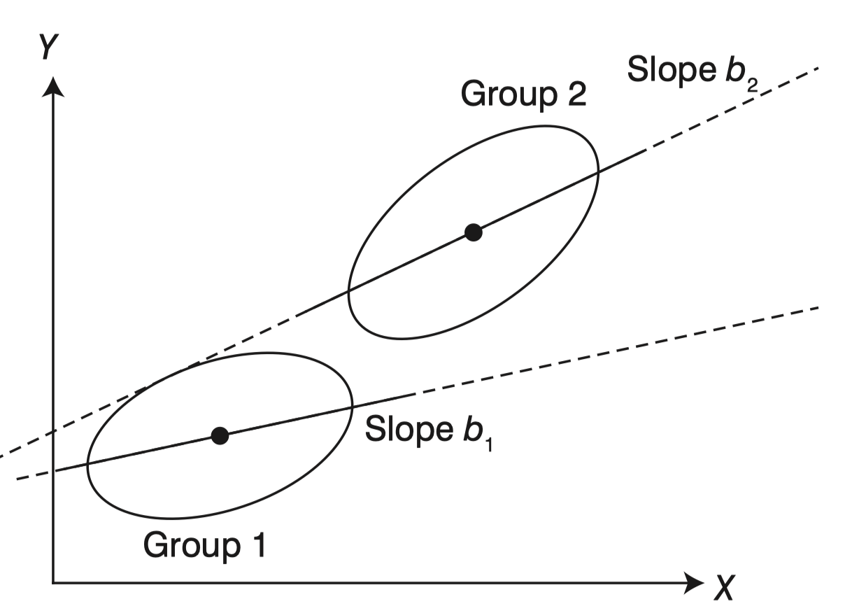
That is because in addition to all previous error terms, we are also adding an error term for each slope.
The dotted lines are fixed slopes. The arrows show the added error term for each random slope.
Random Slope
- The random intercept model can be extended by accommodating one or more predictor variables.
- For example, adding one predictor \(x_{ij}\) to the level 1 model, we obtain:
\[ y_{ij}=\gamma_{00}+\gamma_{10}x_{ij}+U_{0j}+\varepsilon_{ij} \]
Random Slope Level 1
The model can be expressed in 2 different levels, as follows:
Level 1:
\[ y_{ij}=\beta_{0j}+\beta_{1j}x+\varepsilon_{ij} \]
Random Slope Level 2
Level 2:
\[ \beta_{0j}=\gamma_{00}+U_{0j} \]
\[ \beta{ij}=\gamma_{10} \]
The model includes predictors and slopes that relate them to the dependent variable, \(\gamma_{10}\) at level 1 with subscript \(10\). \(\gamma_{10}\) is defined similarly to \(\beta_1\) in the regression model, which is a measure of the effect on \(y\) of a 1-unit change in \(x\).
In addition, in this model \(\gamma_{10}\) and \(\gamma_{00}\) are fixed models, while \(\sigma^2\) and \(\tau^2\) are random models.
Estimation Elaboration
One implication of the model in prior equation is that the dependent variable is influenced by variation between individuals (\(\sigma^2\)), variation between groups (\(\tau^2\)), the average across all groups (\(\gamma_{00}\)), and the effect of the independent variable measured by \(\gamma_{10}\) which is also common to all clusters.
In practice there is no reason that the effect of \(x\) on \(y\) should be common to all clusters, but it is possible that one \(\gamma_{10}\) is common to all clusters. There is a unique cluster effect \(\gamma_{10}+U_{1j}\), where \(\gamma_{10}\) is the average relationship of \(x\) to \(y\) across clusters and \(U_{1j}\) is the variation in the relationship between the two variables. \(\gamma_{10}+U_{1j}\) is assumed to have a mean ) and vary randomly around \(\gamma_{10}\).
Random Slope Model
- The random slope model can be denoted by:
\[ y_{ij}=\gamma_{00}+\gamma_{10}x_{ij}+U_{0j}+U_{1j}x_{ij}+\varepsilon_{ij} \]
From equation above, the fixed model and the random model can be written as follows.
Fixed model: \(\gamma_{00}+\gamma_{10}x_{ij}\)
Random model: \(U_{0j}+U_{1j}x_{ij}+\varepsilon_{ij}\)
The model in the equation above has an interaction between cluster and \(x\), so the relationship between \(x\) and \(y\) is not constant across all clusters.
Centering (1)
- Centering refers to the practice of subtracting the mean of a variable from each individual’s value.
- This implies that the mean for the sample of centered variables is 0, and implies that each individual’s (centered) score represents a deviation from the mean, rather than any meaning its raw value might have.
- In regression, centering is commonly used to reduce co-linearity caused by the inclusion of interaction terms in a regression model.
- Such issues are also important to consider in MLM, where interactions are often used.
Centering (2)
- We saw earlier that the intercept is the value of the dependent variable when the independent variable is set equal to 0.
- In many applications, the independent variable cannot reasonably be 0 (e.g., ESCS), which essentially makes the intercept a value that is needed to fit the regression line but not one that has an easily interpretable value.
- However, when \(x\) has been centered, the intercept takes the value of the dependent variable when the independent variable is at its mean.
- This is a much more useful interpretation for researchers in many situations, and another reason why centering is an important aspect of modeling, particularly in multilevel contexts.
Centering (3)
Data centering is commonly approached by calculating the difference between an individual’s score and the overall mean across the sample.
Another approach, called group mean centering, involves calculating the difference between an individual’s score and the mean of the group they belong to. For example, in schools, overall mean centering would involve finding the difference between each score and the overall mean across the entire school, while group mean centering would entail finding the difference between each score and the mean of the specific school.
The choice between these two approaches should be based on the relationship between variables \(x\) and \(y\).
Overall mean centering allows for the comparison of individuals across the sample, while group mean centering places each individual in their relative position within a group. For instance, using group mean centered ESCS in the analysis for schools means investigating the relationship between students’ relative ESCS scores within their school and their mathematics achievement.
In contrast, overall mean centering would examine the relationship between students’ relative standing in the overall sample on the ESCS and mathematics achievement
Review of Two level MLMs
Previously we learned about the random slope model:
\[ y_{ij}=\gamma_{00}+\gamma_{10}x_{ij}+U_{0j}+U_{1j}x_{ij}+\varepsilon_{ij} \] For example, \(y_{ij}\) is the dependent variable of mathematics achievement, \(x_{ij}\) is the independent variable of ESCS score, and random error at the student and school levels.
Two Part of Random Slope Model
We can extend the random slope model above by including several independent variables at both level 1 and level 2.
In addition to knowing the relationship between ESCS scores and students’ mathematics achievement, we can also find out the extent to which the average ESCS at the school level is related to the students’ ESCS scores.
This model basically has two parts, the first model explains the relationship between individual ESCS (\(x_{ij}\)) and mathematics achievement, and the other model explains the coefficient at level 1 as a function of the level 2 predictor, namely the average ESCS (\(Z_j\)).
Two Part of Random Slope Model
Level 1:
\[ y_{ij}=\beta_{0j}+\beta_{1j}x_{ij}+\varepsilon_{ij} \]
and level 2: \[ \beta_{hj}=\gamma_{h0}+\gamma_{h1}Z_j+U_{hj} \]
- The addition of the above equation is \(y_{h1}Z_{j}\) which represents the slope value for \(y_{h1}\) and the average ESCS score \(Z_j\).
- In other words, the average school achievement is directly related to the coefficient that links students’ ESCS scores to students’ mathematics achievement.
- The two equations at level 1 and level 2 above can be combined into one equation for the following second-level MLM.
Two Part of Random Slope Model
\[ y_{ij}=\gamma_{00}+\gamma_{10}x_{ij}+\gamma_{01}Z_j+\gamma_{1001}x_{ij}Z_j+U_{0j}+U_{1j}X_{ij}+\varepsilon_{ij} \]
- \(\gamma_{00}\) is the intercept,
- \(\gamma_{10}\) is the fixed effect of variable \(x\) (ESCS),
- \(U_{0j}\) represents the random variation of the intercept between groups, and
- \(U_{1j}\) represents the random variation of the slope between groups.
- \(\gamma_{01}\) represents the fixed effect of the level 2 variable (mean ESCS).
- \(\gamma_{11}\) represents the slope and mean of the level 2 variable.
- \(\gamma_{1001}x_{ij}Z_j\) is the cross-level interaction, which is the interaction between level 1 and level 2 predictors. In this case, it is the interaction between student ESCS scores and school mean ESCS scores.